Simple Intro to Natural Language Processing (NLP) with Python
A hopefully simple intro into training a convolutional neural network to identify speech commands using Python, Tensorflow, Librosa, NumPy and Matplotlib.

Download simple-nlp Jupyter Notebook from GitHub Gist.
(Notebook can also be run in Google Colab)
Follow @abayomi185 Star
This tutorial was a submission for my MSc Arificial Intelligence course.
This Jupyter Notebook details the process of importing, sorting and processing a select set of audio commands with corresponding labels, and training a neural network to accurately identify the audio label/command with only the audio data as an input. This forms the fundamentals of artificial intelligent personal assistants such as Apple's Siri, Amazon's Alexa and Google's Assistant. The notebook content is intended to be simple, favouring basic code and coding concepts over abstracted and complex ones.
Objectives:
- Download and import audio dataset
- Shuffle, process and separate dataset into training, validation and testing
- Create and train neural network (NN)
- Test the accuracy of the NN model
The first thing to do is to import all the modules required for this project.
# Built-in Python Modules
# These are mainly for file operations
import glob
import io
import os
import pathlib
import random
import requests
import zipfile
Librosa, Matplotlib and Numpy, popular modules for audio data analysis, various math operations and plotting data.
import librosa
import librosa.display
import matplotlib.pyplot as plt
import numpy as np
TensorFlow, a machine learning library.
import tensorflow as tf
from tensorflow.keras import layers
from tensorflow.keras import models
The next step is to download and extract the speech dataset using built-in python modules
# Dataset directories
audio_dir = pathlib.Path('audio_data')
speech_data = pathlib.Path('audio_data/mini_speech_commands')

if not audio_dir.exists():
  response = requests.get(
      'http://storage.googleapis.com/download.tensorflow.org' +
      '/data/mini_speech_commands.zip'
      )
  zip_file = zipfile.ZipFile(io.BytesIO(response.content))
  zip_file.extractall(audio_dir) # extracted mini_speech_commands
The data has now been download and extracted into the 'audio_data/mini_speech_commands' directory. The audio files can then be organised, shuffled and processed.
speech_commands = []

# Iterate through extracted files to get the spoken commands
for name in glob.glob(str(speech_data) + '/*' + os.path.sep):
  speech_commands.append(name.split('/')[-2])

# Dictionary comprehension to map commands to an integer for quick lookups
speech_commands_dict = {i : speech_commands.index(i) for i in speech_commands}

speech_commands_dict
OUTPUT:
{'down': 4,
 'go': 7,
 'left': 6,
 'no': 1,
 'right': 2,
 'stop': 5,
 'up': 0,
 'yes': 3}
speech_data_list = []

# Iterate through spoken commands to get individual audio files
for name in glob.glob(str(speech_data) + '/*/*'):
  speech_data_list.append(name)

# Seed to ensure shuffled data is repeatable on the same hardware
random.seed(42)
random.shuffle(speech_data_list)
# Labels for corresponding shuffled audio data
speech_data_labels = []

for audio in speech_data_list:
  speech_data_labels.append(os.path.dirname(audio).split('/')[-1])
# Integer representation of labels based on 'speech_commands_dict'
speech_label_int = []

for audio in speech_data_labels:
  speech_label_int.append(speech_commands_dict[audio])
# Compiling all speech data into a list
loaded_speech_data = []

for audio in speech_data_list:
  loaded_speech_data.append(librosa.load(audio, sr=16000))
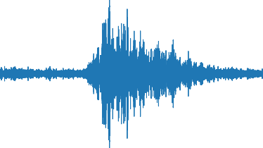
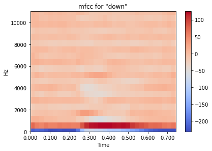
The audio data is processed by converting it to Mel-frequency cepstrum coefficients (MFCCs); a representation of the short-term power spectrum of a sound in the frequency domain.
speech_data_mfcc = []

for loaded_audio in loaded_speech_data:
  speech_data_mfcc.append(librosa.feature
                          .mfcc(
                              loaded_audio[0], loaded_audio[1])
                          )
example_index = 101
librosa.display.specshow(speech_data_mfcc[example_index],
                         x_axis='time', y_axis='hz')
plt.colorbar()
plt.tight_layout()
plt.title(f'mfcc for \"{speech_data_labels[example_index]}\"')
plt.show
# Modified code from source [6] answer
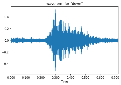
waveform_example = librosa.feature.inverse.mfcc_to_audio(
    speech_data_mfcc[example_index])
librosa.display.waveplot(waveform_example)
plt.tight_layout()
plt.title(f'waveform for \"{speech_data_labels[example_index]}\"')
plt.show
# Modified code from source [6] answer
The compiled, shuffled and processed audio data is then split in the ratio, 70:15:15 for training data, validation data and testing data.
data_length = len(speech_data_list)
data_ratio = {
    'train': 0.7,
    'validate': 0.15,
    'test': 0.15
}
training_ratio = int(data_length*data_ratio['train'])
validation_ratio = int(data_length*data_ratio['validate'])
testing_ratio = int(data_length*data_ratio['test'])

print(f"Dataset Ratio - Training Data: {data_length*data_ratio['train']:.0f}, \
Validation Data: {data_length*data_ratio['validate']:.0f}, Testing Data: \
{data_length*data_ratio['test']:.0f}")
OUTPUT:
Dataset Ratio - Training Data: 5600, Validation Data: 1200, Testing Data: 1200
The audio data is currently of a numpy array data type and needs to be converted to a tensorflow data type in order to use tensorflow functions.
speech_data_as_tensor = []

for index in range(len(speech_data_mfcc)):
  # Inconsistency in array size is rectified by resize the array and
  # filling with zeros
  mfcc_array = np.copy(speech_data_mfcc[index])
  mfcc_array.resize((20,32), refcheck=False)
  speech_data_as_tensor.append(tf.expand_dims(
      tf.convert_to_tensor(mfcc_array), -1))

speech_data_as_tensor[0].shape
OUTPUT:
TensorShape([20, 32, 1])
# Dataset slicing to desired ratios
training_slice = speech_data_as_tensor[:5600]
validation_slice = speech_data_as_tensor[5600: 5600 + 1200]
testing_slice = speech_data_as_tensor[5600 + 1200:]
Tensorflow datasets types are created using the data slices and integer value of the labels
training_dataset = tf.data.Dataset.from_tensor_slices((
    training_slice, speech_label_int[:5600]))
validation_dataset = tf.data.Dataset.from_tensor_slices((
    validation_slice, speech_label_int[5600: 5600+1200]))
testing_dataset = tf.data.Dataset.from_tensor_slices((
    testing_slice, speech_label_int[-1200:]))

batch_size = 10

# Adds a dimension to the dataset that is necessary for
# model fit tensorflow function
training_dataset = training_dataset.batch(batch_size)
validation_dataset = validation_dataset.batch(batch_size)
A Convolutional Neural Network (CNN) Model is created using multiple layers; convolution, relu, pooling, fully-connected
num_labels = len(speech_commands)
norm_layer = layers.Normalization()

# CNN model code as from source [1]
model = models.Sequential([
    layers.Input(shape=(20,32,1)),
    layers.Resizing(32, 32),
    norm_layer,
    layers.Conv2D(32, 3, activation='relu'),
    layers.Conv2D(64, 3, activation='relu'),
    layers.MaxPooling2D(),
    layers.Dropout(0.25),
    layers.Flatten(),
    layers.Dense(128, activation='relu'),
    layers.Dropout(0.5),
    layers.Dense(num_labels),
])
### end of source [1]
Layers of the CNN Model
model.summary()
OUTPUT:
Model: "sequential_1"
_________________________________________________________________
 Layer (type)                Output Shape              Param #
=================================================================
 resizing_1 (Resizing)       (None, 32, 32, 1)         0

 normalization_1 (Normalizat  (None, 32, 32, 1)        3
 ion)

 conv2d_2 (Conv2D)           (None, 30, 30, 32)        320

 conv2d_3 (Conv2D)           (None, 28, 28, 64)        18496

 max_pooling2d_1 (MaxPooling  (None, 14, 14, 64)       0
 2D)

 dropout_2 (Dropout)         (None, 14, 14, 64)        0

 flatten_1 (Flatten)         (None, 12544)             0

 dense_2 (Dense)             (None, 128)               1605760

 dropout_3 (Dropout)         (None, 128)               0

 dense_3 (Dense)             (None, 8)                 1032

=================================================================
Total params: 1,625,611
Trainable params: 1,625,608
Non-trainable params: 3
_________________________________________________________________
# CNN model compile code as from source [1]
model.compile(
    optimizer='Adam',
    loss=tf.keras.losses.SparseCategoricalCrossentropy(from_logits=True),
    metrics=['accuracy'],
)
### end of source [1]
The epoch is determined (the number of training data cycles) and the NN is trained with the training data. This might take some time.
epochs = 10
# Training the Neural Network, this might take some time
measure = model.fit(
    training_dataset,
    validation_data=validation_dataset,
    epochs=epochs,
    callbacks=tf.keras.callbacks.EarlyStopping(verbose=1, patience=3)
    )
Epoch 1/10
560/560 [==============================] - 33s 58ms/step - loss: 1.9472 - accuracy: 0.3936 - val_loss: 1.1123 - val_accuracy: 0.6475
Epoch 2/10
560/560 [==============================] - 33s 59ms/step - loss: 1.0670 - accuracy: 0.6184 - val_loss: 0.8506 - val_accuracy: 0.7050
Epoch 3/10
560/560 [==============================] - 33s 58ms/step - loss: 0.8465 - accuracy: 0.7052 - val_loss: 0.7352 - val_accuracy: 0.7483
Epoch 4/10
560/560 [==============================] - 34s 61ms/step - loss: 0.6994 - accuracy: 0.7489 - val_loss: 0.7521 - val_accuracy: 0.7567
Epoch 5/10
560/560 [==============================] - 33s 59ms/step - loss: 0.6044 - accuracy: 0.7843 - val_loss: 0.6803 - val_accuracy: 0.7792
Epoch 6/10
560/560 [==============================] - 33s 60ms/step - loss: 0.5401 - accuracy: 0.8084 - val_loss: 0.7112 - val_accuracy: 0.7692
Epoch 7/10
560/560 [==============================] - 33s 60ms/step - loss: 0.4433 - accuracy: 0.8427 - val_loss: 0.7109 - val_accuracy: 0.7758
Epoch 8/10
560/560 [==============================] - 34s 60ms/step - loss: 0.4090 - accuracy: 0.8566 - val_loss: 0.7966 - val_accuracy: 0.7808
Epoch 00008: early stopping
metrics = measure.history
# Loss and validation loss
plt.plot(measure.epoch, metrics['loss'], metrics['val_loss'])
plt.legend(['loss', 'val_loss'])
plt.show()
# Modified code from source [1]
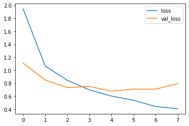
The above plot shows the 'loss' of the model (based on the training dataset) decreasing with epochs, showing that the neural network is learning to identify the speech commands accurately.
The 'val_loss' or validation loss shows that the model starts overfitting at about epoch 3. More audio data would be needed to improve the accuracy of this model.
# Modified CNN model test code from source [1]
test_audio_data = []
test_label_data = []

for audio, label in testing_dataset:
  test_audio_data.append(audio.numpy())
  test_label_data.append(label.numpy())

test_audio_data = np.array(test_audio_data)
test_label_data = np.array(test_label_data)

predicted_values = np.argmax(model.predict(test_audio_data), axis=1)
true_values = test_label_data

test_accuracy = sum(predicted_values == true_values) / len(true_values)
print(f'Test set accuracy: {test_accuracy:.0%}')
### end of modified source [1]
OUTPUT:
Test set accuracy: 74%
As outputted above, the CNN model is able achieve an accuracy in the realm of 75% based on the dataset used.
This has hopefully been a simple introduction to NLP using Python.
Please don't hesitate to ask questions in the comments below or leave a message on the contact page.